What Makes the Best Defensive Footballers?
Analyzing player attributes from FIFA '17 player rankings.
Author: Brian Daisey
Introduction
In football (soccer) as in most sports, the lion's share of the glory goes to the top offensive players. This project shifts the focus onto the defensive element that actually wins championships.
Using detailed player data from the FIFA '17 video game we will examine how defenders match up against the top 1000 players and one another. Then we take a closer look at the defensive players by examining individual attributes and their contribution to the overall player ratings. Hopefully after reading you will have a better idea of which skills are most crucial for the success of defensive footballers!
Outline
- Getting Started
- 1.1 Required Libraries
- 1.2 Dataset Source
- 1.3 Load and View Data
- 1.4 Isolate Top 1000 Players
- 1.5 Isolate Defenders
- Explore Top 1000 Players
- 2.1 Top 1000 Player Breakdown by Position
- 2.2 How Many Defenders in Top 1000?
- Explore Defenders
- 3.1 Defenders by Position
- 3.2 Defenders by Rating
- Begin Defender Analysis
- 4.1 Selection of Attributes
- 4.2 Attributes vs. Rating, Visually
- Reveal Key Attributes with Multiple Linear Regression
- 5.1 Null Hypothesis
- 5.2 Regression with scikit-learn
- 5.3 Regression with statsmodels
- Predict Rating From Attributes with Machine Learning
- 6.1 Predictions with Train/Test Split
- Conclusions
- 7.1 Key Attributes
- 7.2 Prediction of Overall Rating
1. Getting Started
1.1 Required Libraries
- Pandas: used for data display and partitioning
- Matplotlib - pyplot: used for plotting Pandas data into graphs and charts
- Seaborn: provides a high-level interface for graphics on top of Matplotlib
- scikit-learn: very popular machine learning library
- linear-model: used to calculate models for multiple linear regression
- model_selection: used to split up dataset into test and training data and evaluate predictions
- statsmodels - api: used to calculate models and statistics with multple linear regression
import pandas as pd
import matplotlib.pyplot as plt
import seaborn as sns
from sklearn import linear_model
from sklearn import model_selection
from statsmodels import api as sm
1.2 Dataset Source
The dataset used is the ranking for all 17,588 players present in the popular video game FIFA 2017. It contains detailed rankings for all feasible aspects of a players performance, most of which are a ranking out of 100. There is also qualitative data such as Position, Nationality and Club Name. In this project we will be concerned with the quantitave rankings of the players and their postitions.
The dataset was found on Kaggle. There is not much metadata on the Kaggle page, so FIFA Index was used to gain a greater understanding of the attributes present in the dataset and their meaning. Luckily, the FIFA Index pages for individual player statistics very closely match the terms used in the Kaggle dataset.
1.3 Load and View Data
Load .csv file and display the first 5 rows to get a sense of what is contained in the dataset.
fifa = pd.read_csv("FullData.csv")
fifa.head()
Display some basic statistics about the dataset. Since summary statistics are used in the pandas describe() method, only the columns with quantitative data are displayed. Use the 'count' row to get a sense of how complete each column is. There are 17588 players in the dataset in total, so we know that the rows for the specific skill attributes and overall rating are completely populated.
fifa.describe()
Two columns that will be very important for further analysis are 'Rating' and 'Club_Position', so we need to keep only the rows where those columns both have actual values.
fifa = fifa[pd.notnull(fifa['Rating'])]
fifa = fifa[pd.notnull(fifa['Club_Position'])]
fifa.describe()
These columns were nearly complete originally. From the 'count' row in the description of the data above, it appears that only one row was dropped from the dataset.
1.4 Isolate Top 1000 Players
Create a dataframe with only the top 1000 players. This will be based on the 'Rating' field, which contains an overall ranking of each player from 1-100.
# sort descending by Rating
sorted = fifa.copy().sort_values('Rating', ascending=False)

# get top 1000 players
top1000 = sorted.head(1000)
top1000.head()
If you view more than just the head of this dataset, lowest rating among top 1000 is 77. There are more players ranked 77 beyond the top 1000, so this is not a perfect sampling. Since there is no other 'tell-all' attribute, no clear secondary ranking criteria is evident. However, this is not the main focus of the project and this top 1000 set will be suitable for our analysis.
1.5 Isolate Defenders
To isolate the defenders from this dataset, let's first view all the unique position names from the column 'Club_Position'. This column is used over National Position because it has values for all players in the dataset, while National Position only has slightly over 1000 values filled.
fifa['Club_Position'].unique()
To see what these abbreviations actually correspond to, here is an image of football positions on a field:
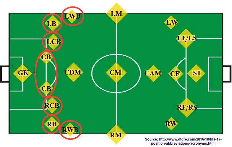
The 7 defensive positions are circled in red above. The abbreviations stand for Left Wingback, Left Back, Left Center Back, Center Back, Right Center Back, Right Back, and Right Wingback.
Now we can make a list of the defensive position acronyms and filter the dataset to return only the defensive players.
def_positions = ['LWB', 'LB', 'LCB', 'CB', 'RCB', 'RB', 'RWB']
defenders = fifa.copy()

#filter based on only records that have the positions present in def_positions above
defenders = defenders[defenders['Club_Position'].isin(def_positions)]
defenders.head()
Verify we still have all 7 defensive positions represented.
defenders['Club_Position'].unique()
From the counts in Rating and individual attributes below, it appears that 2,534 out of the total 17,587 players are listed as defensive players. This yields a large enough dataset for further analysis.
defenders.describe()
2. Explore Top 1000 Players
2.1 Top 1000 Player Breakdown by Position
To find the position breakdown of the top 1000 players we will need a list of all positions and a count of how many players are listed at each. First, we will use Pandas groupby() function to combine all the rows with the same position. Chaining this with count() is what yields our position counts. Finally, sort these counts in a descending manner to view which positions are the most prevalent among the top 1000 players.
by_position = top1000.groupby(top1000['Club_Position']).count().reset_index()
by_position = by_position[['Club_Position','Rating']]
by_position = by_position.sort_values('Rating', ascending=False)
by_position.columns = ['Club_Position','Count']
by_position.head(13)
Unexpected Results!
This is not an ideal result because of the 'Sub' and 'Res' players that are in the dataset. Substitutes and Reserves represent a variety of positions, so this is not informative for our analysis of the breakdown of the top 1000 players by position.
To rectify, we drop all 'Sub' and 'Res' players from the dataset. Then, resample and re-group the top 1000 players.
# drop substitute and reserve players
drop_sub_res = fifa.copy()
drop_sub_res = drop_sub_res[drop_sub_res['Club_Position'] != 'Sub']
drop_sub_res = drop_sub_res[drop_sub_res['Club_Position'] != 'Res']

# sort descending by Rating
sorted = drop_sub_res.copy().sort_values('Rating', ascending=False)

# get new top 1000 players by position
new_top1000 = sorted.copy().head(1000)

by_position = new_top1000.groupby(new_top1000['Club_Position']).count().reset_index()
by_position = by_position[['Club_Position','Rating']]
by_position = by_position.sort_values('Rating', ascending=False)
by_position.columns = ['Club_Position','Count']
by_position.head()
Verify that all 'Sub' and 'Res' players have indeed been dropped from our top 1000 players.
by_position['Club_Position'].unique()
Much better. Let's now plot a histogram of the breakdown of the positions among the top 1000 players for a more visual overview of the distribution.
plt.figure(figsize=(12,6))
plt.title("Top 1000 Players, By Position", fontsize=16)
sns.barplot(data=by_position, x='Club_Position', y='Count')
plt.show()

Obsevations:
- Goalkeepers (GK) are the most represented position among the top 1000 players.
- Strikers (ST), at 3rd most represented, are the only offensive players in the top 12 positions.
- The remaining 10 of the top 12 spots are split between defensive and midfield players.
2.2 How Many Defenders in Top 1000?
To answer this question, use the list of defensive positions generated in Section 1.5. Simply return a count of the number of rows comprising these positions from within the top 1000 players data.
def1000 = new_top1000.copy()
def1000 = def1000[def1000['Club_Position'].isin(def_positions)]
res = def1000.Rating.count()
print("There are {} defenders among the top 1000 players.".format(res))
There are 3 main categories of positions in football: defensive, midfield, and offensive. Subtracting the 119 Goalkeeprs found above, defensive players make up very close to 1/3 of the remaining top 1000 players, so this result is not surprising.
3. Explore Defenders
3.1 Defenders by Position
Let's now take a look at the breakdown of total defensive players by position. Follow the same paradigm as player breakdown in Section 2.1: Group by position, get a count, sort descending, plot!
def_grouped = defenders.groupby(defenders['Club_Position']).count().reset_index()
def_grouped = def_grouped[['Club_Position','Rating']]
def_grouped = def_grouped.sort_values('Rating', ascending=False)
def_grouped.columns = ['Club_Position','Count']
def_grouped
plt.figure(figsize=(12,6))
plt.title("Defensive Player Position Distribution", fontsize=16)
sns.barplot(data=def_grouped, x='Club_Position', y='Count')
plt.show()

Center Backs, Left Wingbacks, and Right Wingbacks have far fewer players listed than the other positions. Perhaps this is due to differing nomenclature across the world for the same positions?
There is also undoubtedly overlap between the RCB, LCB, and CB in that Right and Left Center Backs surely fill in at Center Back from time to time. Also, the positions names may change based on different formations being used throughout the course of a match. This is quickly getting out of depth of my football knowledge, let's proceed.
3.2 Defenders by Rating
Follow the (now familiar) group, count, sort, plot paradigm to get an idea of the ratings distribution for all defensive players.
# group by rating, count, sort
def_by_rating = defenders.groupby(defenders['Rating']).count().reset_index()
def_by_rating = def_by_rating[['Club_Position','Rating']]
def_by_rating = def_by_rating.sort_values('Rating', ascending=False)
def_by_rating.columns = ['Count','Rating']

# plot rating distribution
plt.figure(figsize=(12,6))
plt.title("Defensive Player Rating Distribution", fontsize=16)
sns.barplot(data=def_by_rating, x='Rating', y='Count')
plt.show()

This result is about what you'd expect: many average ratings, with a few very lowly and very highly ranked players. The majority of the players are rated between 60 and 77. Also looks like the data is fairly normally distributed.
4. Begin Defender Analysis
4.1 Selection of Attributes
Now that we have explored the data a bit, we can get down to analysis. The first thing to do is view all of the columns present in the dataset.
# get a list of all the columns
cols = defenders.columns.tolist()

#display all results in a more compact manner
for i,col in enumerate(cols):
    if i%5 ==0:
        print(" ") #new line
    print(col,"   ", end=" ") #do not go to new line after printing each item
This is somewhat overwhelming, especially because there are so many attributes for specific individual player skills.
Luckily, the website FIFA Index maintains detailed information about each player using these same attributes, as well as additional player information such as bios and club membership. FIFA Index can provide us with some guidance moving forward. By viewing one of the individual player pages, we can see that the 34 specific player attributes are grouped into 7 categories. The 5 categories we will focus on are highlighted in red below.
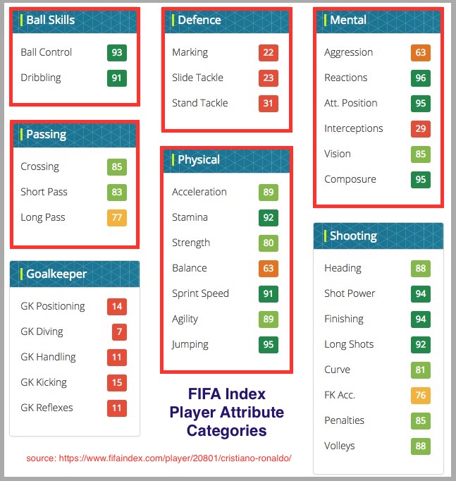
Eliminate Shooting attributes because that does not factor heavily into a defensive player's game. Eliminate Goalkeeper attributes because it is unclear what this category means.
Use the Fifa index to get a list of all the attributes we will be interested in for defensive players.
# lists of attributes by category
ball_skills = ['Ball_Control', 'Dribbling']
passing = ['Crossing','Short_Pass','Long_Pass']
defence = ['Marking', 'Sliding_Tackle', 'Standing_Tackle']
mental = ['Aggression','Reactions','Attacking_Position','Interceptions','Vision','Composure']
physical = ['Acceleration','Stamina','Strength','Balance','Speed','Agility','Jumping']

# list of all defensive attributes
def_group_list = [ball_skills, passing, defence, mental, physical]
# flattens a list of lists
def_attrs_list = [item for sublist in def_group_list for item in sublist]
def_attrs_list
Build a new dataframe from our defensive attributes list, the player ratings overall, position, and player name. Dataframe should have 24 columns: 21 for the attributes and 3 additional for the fields newly added to the list.
new_df_list = ['Name','Club_Position','Rating'] + def_attrs_list

def_with_attrs = defenders.copy()
def_with_attrs = def_with_attrs[new_df_list]
def_with_attrs.head()
Now we will reduce the overall number of attributes by taking the average of the attributes within each category.
Average is used rather than sum because the categories have different numbers of attributes, so this will allow the "category attributes" to all remain on the same scale (out of 100).
# could have used a loop here, but this makes it very clear what is happening
def_with_attrs['Ball_Skills'] = def_with_attrs[ball_skills].mean(axis=1)
def_with_attrs['Passing'] = def_with_attrs[passing].mean(axis=1)
def_with_attrs['Defence'] = def_with_attrs[defence].mean(axis=1)
def_with_attrs['Mental'] = def_with_attrs[mental].mean(axis=1)
def_with_attrs['Physical'] = def_with_attrs[physical].mean(axis=1)
def_with_attrs.head()
View the right-most columns of the above dataframe to see the added categories. Spot-checking the new categories for a couple players reveals that our averages were computed correctly.
Create a new dataframe with just the grouped categories and descriptor columns.
def_grouped_df_list = ['Name','Club_Position','Rating','Ball_Skills','Passing','Defence','Mental','Physical']
def_grouped = def_with_attrs[def_grouped_df_list].reset_index()
def_grouped.head()
Now we have a concise dataframe with the attributes grouped and averaged by their more general categories.
4.2 Attributes vs. Rating, Visually
Create a correlation heatmap to see how the various attributes correlate to Rating and to one another. First need to create a dataframe with just the columns we want to correlate. Then use the pandas function .corr() to create a corellation matrix.
just_cats = def_grouped[['Rating','Ball_Skills','Passing','Defence','Mental','Physical']]
just_cats = just_cats.corr()
just_cats
Plot the correlation matrix onto a heatmap. The heatmap plot within Seaborn makes this very easy to do. Only the first parameter within sns.heatmap is required, the remainder just relate to the display of the plot.
plt.figure(figsize=(12,8))
plt.title("Correlation Heatmap of Rating and Defensive Attributes", fontsize=18)
sns.heatmap(just_cats, cmap=sns.diverging_palette(220, 10, as_cmap=True), square=True, annot=True)
plt.show()

From the heatmap above, we can see that ALL attributes and overall rating are positively correlated to one another using the scale on the right or the annotations in each cell. The more red a box is, the stronger the correlation, and the more blue a box is, the weaker the correlation.
Observations:
- Rating is most strongly correlated with the Defence attribute. This is expected because, after all, we are looking at defensive players only.
- Rating and Mental are also highly correlated.
- Lowest correlation on the whole map is between Physical and Defence. It's more of a mental game to be a defender!
The remainder of our analysis will focus on the top row of this heatmap: how the different attributes affect overall player Rating.
5. Reveal Key Attributes with Multiple Linear Regression
5.1 Null Hypothesis
We are looking at the impacts of 5 different (aggregate) defensive attributes on overall player Rating.
Null Hypothesis: None of the attributes have a noticeable impact on the Rating.
To test the null hypothesis, we will perform Multiple Linear Regression on the dataset using scikit-learn.
5.2 Regression with scikit-learn
Use the dataframe with the grouped attributes for the regression model. Create 2 new dataframes for the features and the target of the regression.
- The features (independent variables) are the attributes Ball Skills, Passing, Defence, Mental, and Physical.
- The target (dependent variable) is the overal player Rating.
grouped_attrs = ['Ball_Skills','Passing','Defence','Mental','Physical']
features = def_grouped[grouped_attrs]
target = def_grouped[['Rating']]
Define X and y for use in scikit-learn's LinearRegression() function. Fit the model.
X = features
y = target['Rating']
lm = linear_model.LinearRegression()
model = lm.fit(X,y)
Get an R-squared score to test how well the variance is explained by the model. Values range from 0 to 1, so the ~0.88 we returned means that almost all the variance is explained by the model.
lm.score(X,y)
Moment of truth! Find the coefficients from the model to see which attributes had the largest impact overall.
sk_coeffs = lm.coef_.tolist()
for attr, coef in zip(grouped_attrs, sk_coeffs):
    print("Attribute: {}, Coefficient: {}".format(attr,coef))
Findings from the heatmap are confirmed. Defence has the most impact on Rating, followed by Mental! Passing actually has a negative impact on Rating, which may or may not be small enough that it is insignificant.
To find out which attributes actually have a meaningful impact (and to test the null hypothesis) we need to observe the p-values. This is beyond the capability of scikit-learn.
5.3 Regression with statsmodels
It is possible to reuse the features (X) and target (y) variables created in Section 5.2, so setting up a model in statsmodels is very simple. The only thing to note is that we have to add a constant in statsmodels manually. We want to use one because we know that our Rating data does not go all the way to zero.
This model uses the method of Ordinary Least Squares (OLS) to estimate our parameters. OLS basically aims to minimize the sum of the squared distances between the actual values in the dataset and the predicted values generated by the regression line. More information about Ordinary Least Squares can be found here.
sm_y = y
sm_X = X

#add a constant to the features
sm_X = sm.add_constant(X)

# use Ordinary Least Squares
OLS_model = sm.OLS(y,X).fit()
OLS_model.summary()
Looking at the coefficients above ('coef' column in the middle chart), it is clear that Defence and Mental again have the most impact on player Rating.
It is interesting to note that the impact from Passing is indeed negligible. From the p-values above ('P>|t|' column in the middle chart) we can see that it is the only one above a critical value of 5% (p-value of 0.05). The remainder of the p-values are well below 0.05, which means they have significance within the model.
This means that we reject the null hypothesis because clearly the player attributes to contribute to the overall player Rating.
A point of concern is the R-squared result of 0.999. This indicates that we may have overfit the model. We will see how our data works with training and test sets in the next section, which will lend some insight about overfitting.
Note: This tutorial was invaluable in performing these two models of Multiple Linear Regression.
6. Predict Rating From Attributes with Machine Learning
6.1 Predictions with Train/Test Split
Reuse X and y again from scikit-learn regression for our model selection. Here we will split up the dataset into training and testing data for both variables. X_train and Y_train are used to generate (train) the multiple linear regression model. Then, the X_test data (grouped attributes) is used with the model to make predictions for the expected Ratings. These predictions are then compared with the actual Rating values (found in y_test).
Test/train split is up to the user, but the majority of the dataset should be used to train the model. Here we will use 80% of the data for training and 20% for testing results.
# create training and testing data from same X and y used in regression above
X_train, X_test, y_train, y_test = model_selection.train_test_split(X, y, test_size=0.2)

# create and fit the model
lm = linear_model.LinearRegression()
model = lm.fit(X_train, y_train)

# generate predictions for player Rating to compare with y_test data
predictions = lm.predict(X_test)

# display first 10 results of our predicted player Ratings.
predictions[0:10]
Plot the predicted values from the model against the actual values from the dataset (y_test).
Add an identity line for predictions = y_test. This identity line will inform us how closely the predictions are to the actual rating values. The better the predictions, the more closely the plotted points will follow the identity line.
plt.figure(figsize=(8,8))
plt.title("Predicted vs. Actual Values for Player Rating", fontsize=16)
plt.scatter(y_test,predictions)
plt.plot(y_test, y_test, color="Red") # identity line y=x
plt.xlabel("Actual Values")
plt.ylabel("Predicted Values")
plt.show()

From the plot above it is clear that the model predicted the player Ratings very well for the test data.
The model also provides a score of the actual accuracy (1 is perfect).
print("Accuracy (scale of 0 to 1): {}".format(model.score(X_test, y_test)))
This is a suspiciously high accuracy score for the model. Rather than overfitting the model, as suspected in section 5.3, it likely has to do with the nature of the dataset itself. This is discussed further in Section 7 below.
Note: This tutorial was followed to carry out the train/test split and plotting of the results. It is by the same author as the regression tutorial above and both are very highly recommended for learning more about these topics.
7. Conclusions
7.1 Key Attributes
From the heatmap (Section 4.2) and two multiple linear regression models (Section 5.2 and 5.3) we discovered that player attributes do indeed affect the overall player Rating. Not surprisingly because we looked at defensive players, the Defence attribute plays the biggest role in determining overall Rating. More interestingly, the Mental category is the second-strongest contributor to overall Rating. From the OLS model and p-values in Section 5.3, we see that Physical also contributes as does Ball Skills (to a much lesser extent). Passing does not contribute to the model in a significant way.
All the virtual football managers out there should take note of how much more important the Mental attributes are than Physical ones!
It is surprising that Passing does not contribute to the model because you would expect that passing well to clear the ball out of the defensive portion of the field would be an important contributor to the overall rating of a defensive player.
7.2 Prediction of Overall Rating
The predictions of the model so closely matched the actual player ratings that it raises suspicion. After doing some research about why the R-squared value can be too high, overfitting the model is not likely the cause. Overfitting occurs when there are too many features (player attributes) in the model when compared with the number of observations. When this happens, the regression model "bends" too closely to the actual points and reflects the noise in the data rather than actually generalizing the overall population. It is always discretionary, but using 5 attributes for a sample size of over 2500 observations seems reasonable.
The cause of the very accurate model (and suspiciously high R-squared value) is likely due more to the structure of the dataset itself. Rather than being generated from real-world observations, or calculated from joining disparate datasets, the overall player Rating is DERIVED from the attributes themselves. While we do not know the actual weights and algorithms applied to the individual attributes to generate player Rating, it is probable that the creators of FIFA '17 mostly used these attributes when computing overall player rating. This likely explains why virtually all of the variance is explained by our linear regression model and why the predicted Ratings were so close to the actual Ratings.
Thank you for reading! Any comments/criticisms of methodology, analysis, display, clarity of writing, or lack of actual football knowledge are warmly welcomed!